library(ggplot2)
library(patchwork)Normal Distribution
Required Packages
theme_set(theme_bw())
theme_replace(panel.grid.minor = element_blank(),
              panel.grid.major = element_blank())
Normal Distribution
One of the most important and widely used continuous distribution is the Normal distribution, or Gaussian distribution.
Let \(X \sim N(\mu,\sigma)\) be a random variable following a normal distribution with mean \(\mu\) and standard deviation \(\sigma\). In R, the following functions described in the table below, allows us to summarize the function relating to the normal distribution
| Function | Description |
|---|---|
| dnorm | Normal density (Probability Density Function) |
| pnorm | Normal distribution (Cumulative Distribution Function) |
| qnorm | Quantile function of the Normal distribution |
| rnorm | Normal random number generation |
By default, all of the functions above consider the standard Normal distribution, which has a mean of zero and a standard deviation of one, \(X \sim N(0,1)\)
dnorm
The density function for a normal distribution with mean \(\mu\) and standard deviation \(\sigma\) is
\[ f(x) = \frac{1}{\sigma \sqrt{2\pi}} \exp{\left( -\frac{1}{2\sigma^2 }(x-\mu)^2 \right)} \] for \(-\infty < x < \infty\)
We can use dnorm() function to calculate the density function, i.e \(f(x)\), for a grid of \(x\) values from any normal distribution with mean \(\mu\) and standard deviation \(\sigma\)
For example, we can calculate \(f(0)\) from a standard normal distribution
dnorm(x = 0,mean = 0,sd = 1)#> [1] 0.3989423Consider evaluating \(f(x)\) for \(x \in [1,10]\) with mean 1 and standard deviation of 3
dnorm(x=1:10,mean = 1,sd = 3)#> [1] 0.132980760 0.125794409 0.106482669 0.080656908 0.054670025 0.033159046
#> [7] 0.017996989 0.008740630 0.003798662 0.001477283pnorm
The pnorm() function gives the Cumulative Distribution Function (CDF) of the Normal distribution, which is the probability that the variable \(X\) takes a value less than or equal to \(x\). Mathematically, \(F_X(x) = P(X \leq x)\).
For any continuous distribution \(P(X = x)=0\), so equivalently the CDF is \(P(X \leq x) = P(X < x)\).
Consider the standard normal distribution, since this distribution is symmetrical centered around \(\mu=0\) then \(P(X \leq 0) = 0.5\). We can verify this result using pnorm as follows
pnorm(0,mean = 0, sd = 1)#> [1] 0.5Example: Suppose \(X\) is the SAT-M score which has a normal distribution with a mean of 507 and standard deviation of 111. What is the probability of scoring less than 700 on the SAT-M?
Show Code
prob1 <- round(pnorm(700, mean=507, sd=111) * 100,2)
plt1 <- ggplot(data.frame(x = c(150,900)), aes(x)) +
  stat_function(fun = dnorm,
                geom = "line",
                xlim = c(150,900),
                args = list(mean = 507,sd = 111)) +
  stat_function(fun = dnorm,
                geom = "area",
                fill = 'steelblue',
                alpha =0.3,
                xlim = c(150, 700),
                args = list(mean = 507,sd = 111))+
  annotate("text", x = 510, y = 0.0015,
           label = paste0(prob1,'%'),
           size = 8)+
  geom_vline(xintercept = 700,linetype =2)+
  labs(x = '',y= 'Density')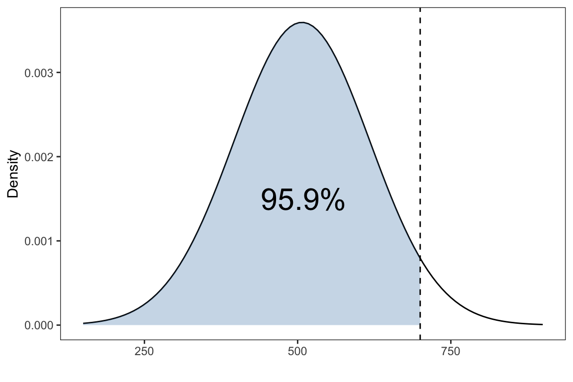
That is \(P(X < 700)\),
pnorm(700, mean=507, sd=111)#> [1] 0.9589596What about the probability of scoring greater than 700?
Show Code
prob2 <- round(pnorm(700, mean=507, sd=111,
                     lower.tail = FALSE)*100,2)

p2 <- ggplot(data.frame(x = c(150,900)), aes(x)) +
  stat_function(fun = dnorm,
                geom = "line",
                xlim = c(150,900),
                args = list(mean = 507,sd = 111)) +
  stat_function(fun = dnorm,
                geom = "area",
                fill = 'steelblue',
                alpha =0.3,
                xlim = c(700, 900),
                args = list(mean = 507,sd = 111))+
  annotate("text", x = 738, y = 0.00017,
           label = paste0(prob2,'%'),
           size=4.7)+
  geom_vline(xintercept = 700,linetype =2)+
  labs(x = '',y= 'Density')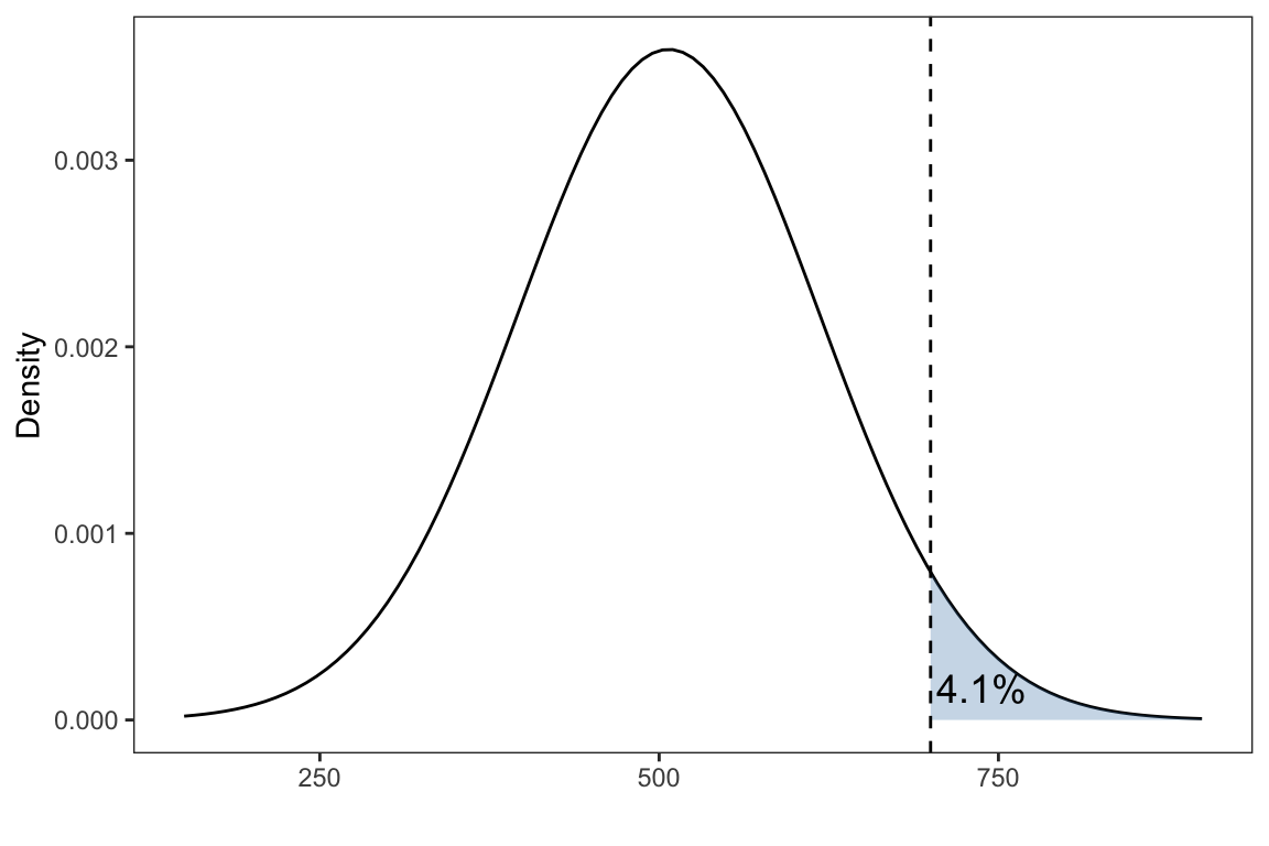
We are interested \(P(X > 700)\), which can be obtained through \(P(X > 700) = 1- P(X \leq 700)\)
1-pnorm(700, mean = 507, sd = 111)#> [1] 0.04104036Alternative, pnorm() has an argument lower.tail=TRUE (by default). If lower.tail=TRUE, the probabilities \(P(X \leq x)\) are returned. Otherwise, if lower.tail=FALSE, \(P(X > x)\) are returned
pnorm(700, mean = 507, sd = 111, lower.tail = FALSE)#> [1] 0.04104036The Empirical rule (also known as the 68-95-99.7 rule) is a statistical rule stating that for a normal distribution, where most of the data will fall within three standard deviations of the mean. The empirical rule can be broken down into three parts: 68% of data falls within the first standard deviation from the mean (blue shaded region). 95% fall within the 2nd standard deviations (up to the green shaded region). 99.7% fall within third standard deviation (up to the red shaded region)
Show Code
x_limits <- c(-4,4)plot_shaded_normal <- function(shade_limits,percent_display,
annotate_x_label,annotate_y_label,
x_limits = c(-4,4),
fill = 'steelblue',
alpha = 0.3,annotate_label_size=4.5){
plt <- ggplot(data.frame(x = x_limits), aes(x)) +
stat_function(fun = dnorm,geom = "line",xlim = x_limits) +
stat_function(fun = dnorm,geom = "area",fill = fill,alpha =alpha,
xlim = shade_limits)+
labs(x = '',y= 'Density')+
annotate("text", x = annotate_x_label, y = annotate_y_label,
label = paste0(percent_display,'%'),
size=annotate_label_size)+
scale_x_continuous(name = '',limits = x_limits,
breaks = x_limits[1]:x_limits[2])
return(plt)
}plots <- plot_shaded_normal(shade_limits = c(-1,1),
percent_display = 68,
annotate_x_label = 0.1,annotate_y_label = 0.15)+
plot_shaded_normal(shade_limits = c(-2, 2),fill='green',
percent_display = 95,
annotate_x_label = 0,annotate_y_label = 0.15)+
plot_shaded_normal(shade_limits = c(-3, 3),fill='red',
percent_display = 99.7,
annotate_x_label = 0.1,annotate_y_label = 0.15)+
plot_annotation(title = '68–95–99.7 Rule')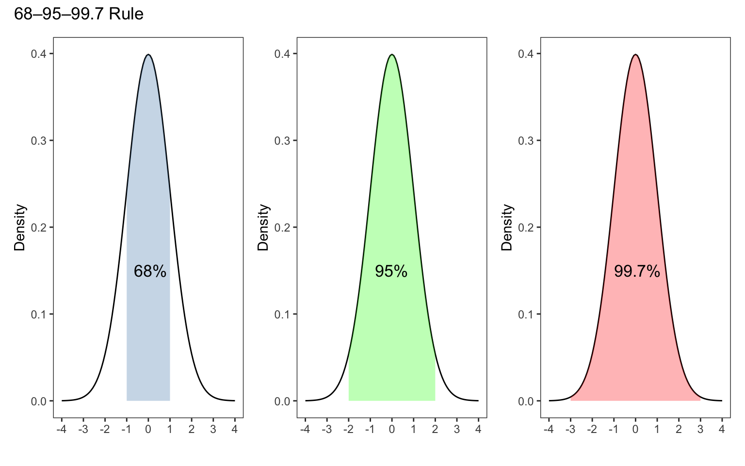
We can easily verify these results using pnorm. Assuming a standard Normal distribution if we were one standard deviation away from the mean then
pnorm(1)-pnorm(-1)#> [1] 0.6826895If we were two standard deviations away from the mean
pnorm(2) - pnorm(-2)#> [1] 0.9544997and lastly, three standard deviations away from the mean
pnorm(3) - pnorm(-3)#> [1] 0.9973002qnorm
The function qnorm() returns the value of the inverse cumulative density function (CDF) of the normal distribution with specified mean \(\mu\) and standard deviation \(\sigma\).
Let \(F_X(x) = P(X \leq x)\) be the CDF of the normal distribution, and suppose it returns the probability \(p\), i.e, \(F_X(x) = p\). The inverse of the CDF or (quantile function) tells you what \(x\) would make \(F_X(x)\) return some probability \(p\);
\[F_X^{-1}(p) = x\] For example, for the standard normal distribution \(F_X(0)=P(X \leq 0) = 0.5\). That is, the value of \(x\) or (quantile) which gives us a cumulative probability of 0.5 is \(x=0\).
Therefore, we can use the qnorm() function to find out what value of \(x\) or (quantile) gives us a a cumulative probability of \(p\). Hence, the qnorm function is the inverse of the pnorm function
Show Code
x_limits <- c(-4,4)

p1 <- ggplot(data.frame(x = x_limits), aes(x)) +
  stat_function(fun = dnorm,
                geom = "line",
                xlim = x_limits) +
  stat_function(fun = dnorm,
                geom = "area",
                fill = 'steelblue',
                alpha =0.3,
                xlim = c(-4, 0))+
  geom_vline(xintercept = 0,linetype=2,color = '#cf5d55')+
  labs(x = '',y= 'Density')+
  annotate('text', x = -0.65, y = 0.17,
           parse =TRUE,
           label = paste0(
             expression('F'[x]),'(0)==0.5') )+
  annotate('text',x = 0.77, y = 0.41,
           parse =TRUE,
           label = paste0(
             expression('F'[x]^{-1}),' *(0.5)==0'),
           color = '#cf5d55')+
  scale_x_continuous(name = '',limits = x_limits,
                     breaks = -4:4)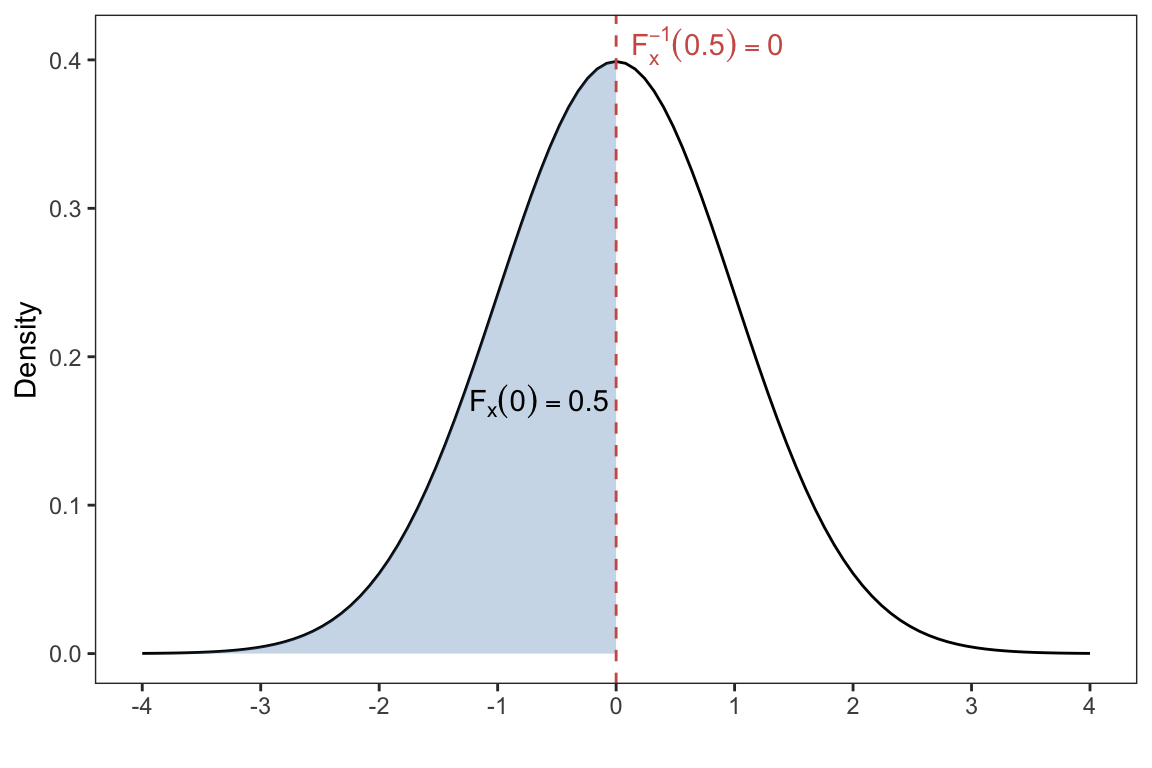
qnorm(p=0.5)#> [1] 0Going back to our example of the SAT-M scores. Suppose \(X\) is the SAT-M score which has a normal distribution with a mean of 507 and standard deviation of 111. Recall the probability of obtaining a score less than 700 on the SAT-M was \(P(X < 700) = 0.9589596\). Therefore, if we were interesting in finding the score or (quantile) which gives us a cumulative probability of roughly 96% we can use qnorm as follows:
qnorm(0.9589596, mean=507, sd=111)#> [1] 700We should see that the output value is exactly 700.
rnorm
The rnorm function generates \(n\) observations from a Normal distribution with mean \(\mu\) and standard deviation \(\sigma\).
We specify a seed for reproducibility,
set.seed(10)Let’s start by generate 10 random observations from a standard normal distribution
rnorm(10, mean = 0, sd = 1)#> [1] 0.01874617 -0.18425254 -1.37133055 -0.59916772 0.29454513 0.38979430
#> [7] -1.20807618 -0.36367602 -1.62667268 -0.25647839or equivalently,
rnorm(10)#> [1] 1.10177950 0.75578151 -0.23823356 0.98744470 0.74139013 0.08934727
#> [7] -0.95494386 -0.19515038 0.92552126 0.48297852We can specify a different mean and standard deviation
rnorm(10, mean = 10, sd = 2)#> [1] 8.807379 5.629426 8.650268 5.761878 7.469604 9.252677 8.624889 8.255682
#> [9] 9.796478 9.492439In the following plot we generate \(n=100,1000,10000\) random observations from a standard normal distribution. If we increase the number of observations, we see the data will approach the true Normal density function
Show Code
plot_random_normal <- function(n_samples, mean = 0, sd = 1,
                               fill = 'steelblue', alpha = 0.3,
                               bins = 30, density_linewidth = 1.2,
                               density_linetype = 2){

  plt <- ggplot(data = data.frame(x=rnorm(n_samples,mean = mean, sd = sd),
                                  n_samples),aes(x))+
    geom_histogram(aes(y = after_stat(density)),
                   colour = 1, fill = fill,
                   alpha = alpha,
                   bins=bins) +
    geom_density(linewidth = density_linewidth,
                 linetype = density_linetype,
                 colour = 2)+
    labs(x= '',y = 'density')+
    facet_grid(~n_samples)
  return(plt)
}
plots <- plot_random_normal(n_samples = 100)+
plot_random_normal(n_samples = 1000)+
plot_random_normal(n_samples = 10000)+
plot_layout(ncol=3)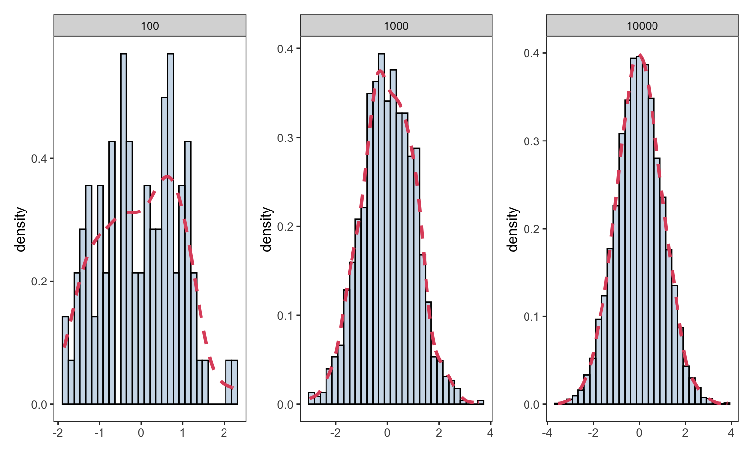
Standardizing Values
The normal model \(N(0,1)\) is called the standard normal distribution, and it is the default model used when working with (.)norm functions
A \(z\)-score, also known as a standard score, quantifies the number of standard deviations a data point is from the mean of a distribution. This can be useful for comparing and analyzing data across different scales or distributions, providing a standardized way to assess the relative position of a particular value within a dataset
For example, consider a scenario where you are comparing the performance of students in two different subjects, one with scores ranging from 0 to 100 and another with scores ranging from 0 to 50. Without standardization, it can be challenging to assess which student has performed relatively better across both subjects.
The \(z\)-score of a particular value is defined as \[ z = \frac{\text{value} - \text{mean}}{\text{standard deviation}} \] If the values in their original units of measurement follow a normal distribution, then the \(z\)-scores will follow a standard normal distribution
Recall the SAT-M scores example: Suppose \(X\) is the SAT-M score which has a normal distribution with a mean of 507 and standard deviation of 111. What is the probability of scoring less than 700 on the SAT-M?
pnorm(700, mean = 507, sd = 111)#> [1] 0.9589596We can also compute this quantity with the \(z\)-score with respect to the standard normal distribution \[ \begin{align*} z &= \frac{\text{value} - \text{mean}}{\text{standard deviation}} \\[10pt] z &= \frac{700 - 507}{111} \\[10pt] z &= 1.738739 \end{align*} \]
z <- (700-507)/111
pnorm(z)
#> [1] 0.9589596Show Code
prob2 <- round(z * 100,2)
p2 <- ggplot(data.frame(x = c(-4,4)), aes(x)) +
  stat_function(fun = dnorm,
                geom = "line",
                xlim = c(-4,4),
                args = list(mean = 0,sd = 1)) +
  stat_function(fun = dnorm,
                geom = "area",
                fill = 'red',
                alpha =0.3,
                xlim = c(-4, z),
                args = list(mean = 0,sd = 1))+
  annotate("text", x = (510-507)/111, y = 0.15,
           label = paste0(prob1,'%'),
           size = 8)+
  geom_vline(xintercept = z,linetype =2)+
  labs(x = '',y= 'Density')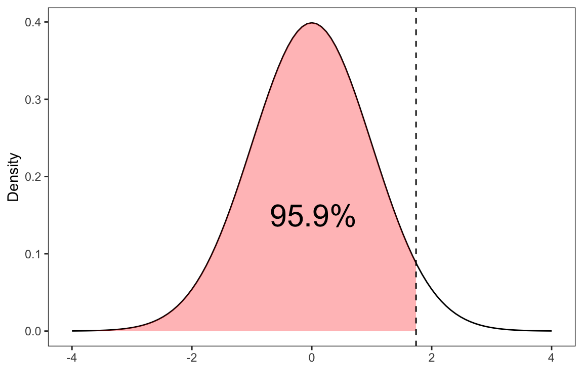
By standardizing the scores, we shift from calculating \(P(X < 700)\) where the units are in SAT-M scores to equivalently computing \(P(Z < 1.738739)\). This represents the number of standard deviations a data point is from the mean of the distribution. By standardizing we can now compare these results with say scores obtained from an english SAT exam on the same scale