Simulation-Based Test of Significance

Required Packages

library(openintro)
library(palmerpenguins)
library(mosaic)
library(ggplot2)

theme_set(theme_bw())
theme_replace(panel.grid.minor = element_blank(),
              panel.grid.major = element_blank())

---

Comparing two proportions

From the openintro package we consider the sten30 dataset. An experiment that studies effectiveness of stents in treating patients at risk of stroke with some unexpected results, this dataset represent the results 30 days after stroke

stent30 <- openintro::stent30

#> Rows: 451
#> Columns: 2
#> $ group   <fct> treatment, treatment, treatment, treatment, treatment, treatme…
#> $ outcome <fct> stroke, stroke, stroke, stroke, stroke, stroke, stroke, stroke…

We are interesting in testing if the probability of having a stroke is different for those in the control and treatment group. The null and alternative hypotheses are given by \[ \begin{align*} H_0: \pi_1 &= \pi_2 \\[5pt] H_a: \pi_1 &\neq \pi_2 \end{align*} \]

observed_tbl <- tally(outcome~group,data=stent30 ,format='proportion')

The observed statistic is the difference in proportion of individuals who did get a stroke under the treatment and control groups

observed_diff <- observed_tbl['stroke','treatment'] - observed_tbl['stroke','control']

observed_diff

#> [1] 0.09005271

Below is a for loop that will simulate the null distribution for our test statistic we will use to test our hypothesis

set.seed(234)
iters <- 5000
diff_proportions <- numeric(iters)

for(i in 1:iters){
  group_shuffle_i <- sample(stent30$group)
  cond_props_i <- tally(stent30$outcome~group_shuffle_i,format = 'proportion')
  
  diff_proportions[i] <- cond_props_i['stroke','treatment'] - cond_props_i['stroke','control']
}

Show Code

sampling_dist <- ggplot(data.frame(diff_proportions),
                        aes(diff_proportions))+
  geom_histogram(fill = 'steelblue',alpha = 0.3,
                 color = 'black',bins=25)+
  geom_vline(xintercept = observed_diff,linetype = 2,
             color ='red')+
  geom_vline(xintercept = -observed_diff,linetype = 2,
             color ='red')+
  labs(title = 'Sampling distribution',
       subtitle = '',
       x = 'Sample Difference of Proportions',y = '')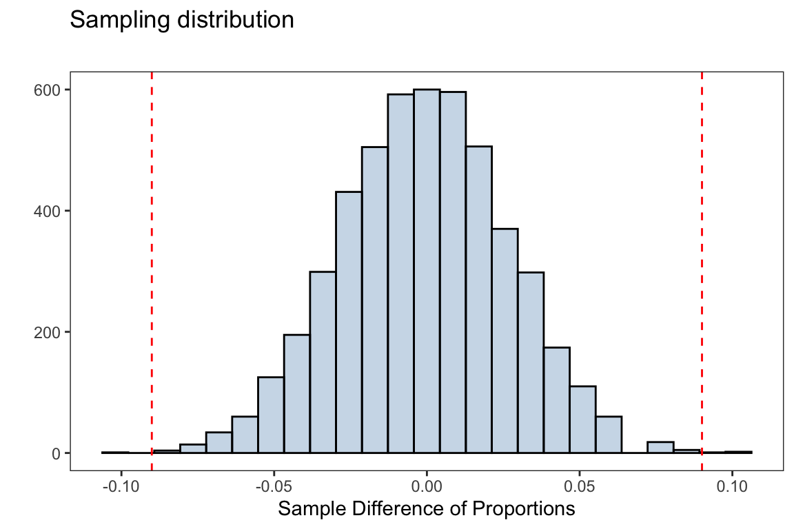

Using our null distribution, we can decide on the strength of evidence for or against the null hypothesis. The simulation-based \(p\)-value is then computed as

mean(abs(diff_proportions) >= observed_diff)

#> [1] 8e-04

Using a significance level of \(\alpha=0.05\), we have enough evidence in favor of the alternative hypothesis. That is, we reject the null hypothesis and suggest there is a difference in proportions of patients getting a stroke under the control and treatment group.

Comparing two means

Using the penguins dataset from the package palmerpenguins, in this portion of the tutorial we are interested in whether the average body mass (in grams) of Adelie type penguins is less than that of Chinstrap penguins

We will test this comparing the mean body mass between Adelie and Chinstrap penguins using a simulation-based approach

First, we remove missing data concerning the two variables of interest species and body_mass_g

subset_filter <- is.na(penguins$species)|is.na(penguins$body_mass_g)| penguins$species == 'Gentoo'

penguins_dat will be the dataset without missing values for the species and body_mass_g variables

penguins_dat <- subset(penguins,!subset_filter)

observed_means <- mean(body_mass_g ~ species, data = penguins_dat)

The observed statistic is the difference in means of Adelie type penguins and Chinstrap penguins

observed_means_diff <- observed_means['Adelie']-observed_means['Chinstrap']
observed_means_diff

#>    Adelie 
#> -32.42598

The null and alternative hypotheses are given by

\[ \begin{align*} H_0: \mu_{\text{adelie}} = \mu_{\text{Chinstrap}} \\ H_a: \mu_{\text{adelie}} < \mu_{\text{Chinstrap}} \end{align*} \]

Below is a for loop that will simulate the null distribution for our test statistic we will use to test our hypothesis

iters <- 5000
diff_means <- numeric(iters) 
set.seed(123)

for (i in 1:iters){
    species_shuffle_i <- sample(penguins_dat$species)
    means_i <- mean(body_mass_g ~ species_shuffle_i, data=penguins_dat)
    diff_means[i] <- means_i[1] - means_i[2]
}

Show Code

sampling_dist <- ggplot(data.frame(diff_means),
                        aes(diff_means))+
  geom_histogram(fill = 'steelblue',alpha = 0.3,
                 color = 'black',bins=30)+
  geom_vline(xintercept = observed_means_diff,linetype = 2,
             color ='red')+
  labs(title = 'Sampling distribution',
       subtitle = '',
       x = 'Sample Difference of Means',y = '')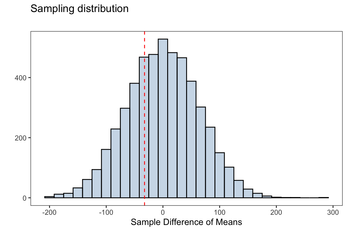

Using our null distribution, we can decide on the strength of evidence for or against the null hypothesis. The simulation-based \(p\)-value is then computed as

mean(diff_means <= observed_means_diff)

#> [1] 0.3098

Using a significance level of \(\alpha=0.05\), we do not have enough evidence in favor of the alternative hypothesis. That is, we fail to reject the null hypothesis and cant suggest the average body mass of Adelie type penguins is less than that of a Chinstrap penguin