Simple Linear Regression

Required Packages

library(palmerpenguins)
library(mosaic)
library(ggplot2)

theme_set(theme_bw())
theme_replace(panel.grid.minor = element_blank(),
              panel.grid.major = element_blank())

Introduction to Simple Linear Regression

Simple linear regression is a statistical method which allows us to predict a quantitative outcome \(y\) on the basis of a single predictor variable \(x\).

• Sometimes \(x\) is regarded as the predictor, explanatory, or independent variable.

• Similarly, \(y\) is regarded as the response, outcome, or dependent variable

We will only use predictor and response to denote our variables of interest. The goal is to define a statistical model that defines the response variable (y) as a function of the predictor (x) variable. Once, we built a statistically significant model, it’s possible to use it for predicting outcomes on the basis of new predictor values.

Below are all the numerical variables in our dataset

colnames(Filter(is.numeric,penguins))

[1] "bill_length_mm"    "bill_depth_mm"     "flipper_length_mm"
[4] "body_mass_g"       "year"             

For our simple linear regression model, we will consider the body mass (grams) of the penguins as the response variable and the length of the length of the the penguin’s flipper (millimeters) as our single predictor variable

Our model takes the form \[ (body\_mass_g) = \beta_0 + \beta_1 \cdot (flipper\_length_{mm}) + \epsilon \] where

• \(\beta_0\) is the intercept of the regression line, (when flipper_length_mm =0)
• \(\beta_1\) is the slope of the regression line
• \(\epsilon\) is the error terms

For simplicity we will remove any missing data from our variables of interest

missing_dat <- is.na(penguins$flipper_length_mm)|is.na(penguins$body_mass_g)

penguins_dat will be the dataset without missing values for the flipper_length_mm and body_mass_g variables

penguins_dat <- subset(penguins,!missing_dat)

For syntax purposes, we create variables for flipper_length_mm and body_mass_g to avoid using penguins_dat$ throughout the tutorial

flipper_length_mm <- penguins_dat$flipper_length_mm
body_mass_g <- penguins_dat$body_mass_g

We can view the relationship between body_mass_g and flipper_length_mm using a scatter plot

plot(flipper_length_mm,body_mass_g,
     xlab = 'Flipper length (mm)',
     ylab = 'Body mass (grams)')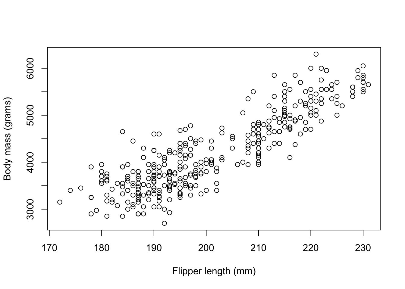

SLR in R

simple_lm <- lm(body_mass_g ~ flipper_length_mm)
simple_lm

Call:
lm(formula = body_mass_g ~ flipper_length_mm)

Coefficients:
      (Intercept)  flipper_length_mm  
         -5780.83              49.69  

The model can be written as body_mass_g = -5780.83 + 49.69*flipper_length_mm, this is our line of best fit. We can then plot our line of best fit as shown below

plot(flipper_length_mm,body_mass_g,
     xlab = 'Flipper length (mm)',
     ylab = 'Body mass (grams)')
abline(simple_lm,col = 'red',lwd =2)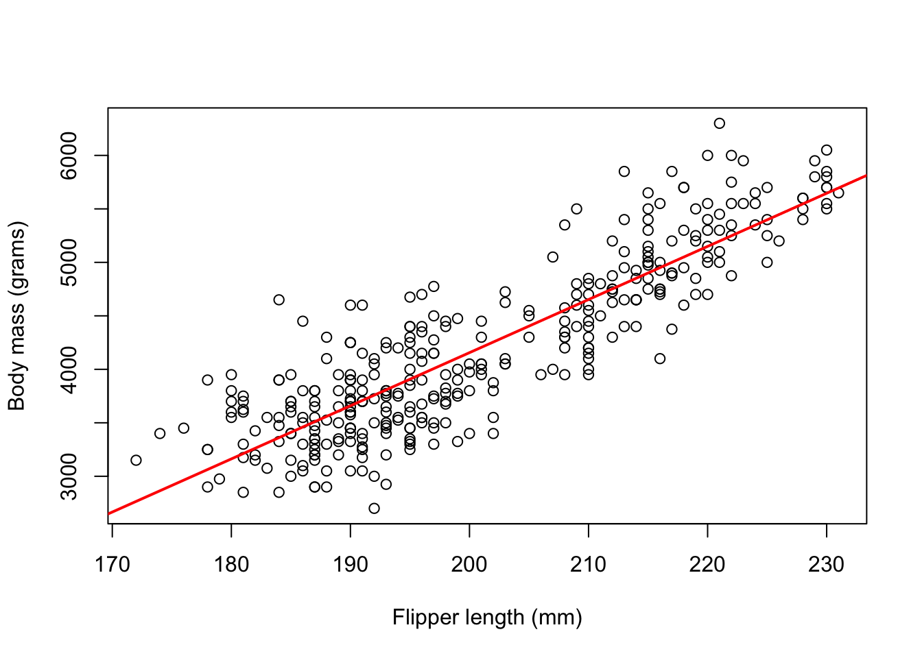

Moreover, we can use the summary() function to quickly check whether our predictor is significantly associated with the response variable. If so, we can further assess how well our model fits our actual data by utilizing metrics provided by the summary output

Model Summary

lm_summary <- summary(simple_lm)
lm_summary

Call:
lm(formula = body_mass_g ~ flipper_length_mm)

Residuals:
     Min       1Q   Median       3Q      Max 
-1058.80  -259.27   -26.88   247.33  1288.69 

Coefficients:
                   Estimate Std. Error t value Pr(>|t|)    
(Intercept)       -5780.831    305.815  -18.90   <2e-16 ***
flipper_length_mm    49.686      1.518   32.72   <2e-16 ***
---
Signif. codes:  0 '***' 0.001 '**' 0.01 '*' 0.05 '.' 0.1 ' ' 1

Residual standard error: 394.3 on 340 degrees of freedom
Multiple R-squared:  0.759, Adjusted R-squared:  0.7583 
F-statistic:  1071 on 1 and 340 DF,  p-value: < 2.2e-16

The ’*’ symbols indicate the level of significance for the respective term. The significance codes below the line shows the definitions for the level of significance; one star means \(0.01 < p < 0.05\), two stars mean \(0.001 < p < 0.01\), and similar interpretations for the remaining symbols

Breaking down the summary output, it contains the following components (Extract using $ operator)

Call

The function (formula) used to compute the regression model

lm_summary$call

lm(formula = body_mass_g ~ flipper_length_mm)

Residuals

The difference between predicted values for the response variable using our constructed model and the observed response values from our original data. Mathematically, \[ r_i = y_i - \hat{y}_i \]

If the residual is

• Positive: The predicted value was an underestimate of the observed response
• Negative: The predicted value was an overestimate of the observed response
• Zero: The predicted value is exactly the same as the observed response

Show Code

dat <- cbind.data.frame(flipper_length_mm,body_mass_g)

p1 <- ggplot(dat, aes(x = flipper_length_mm, y = body_mass_g)) +
  geom_smooth(method = "lm", se = FALSE, 
              color = "lightgrey",formula = 'y~x') +
  geom_segment(aes(xend = flipper_length_mm, 
                   yend = predict(simple_lm)), alpha = .2) +
  geom_point(aes(color=residuals(simple_lm))) +
  guides(color = 'none') + 
  scale_color_gradient2(low = "blue", mid = "white", high = "red") +
  labs(x = 'Flipper length (mm)',
       y = 'Body mass (grams)')+
  theme_bw()+
  theme(panel.grid.minor = element_blank(),
        panel.grid.major = element_blank())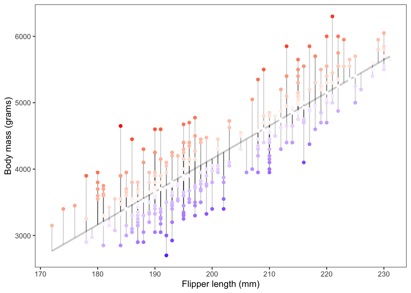

The figure above shows the magnitude of the resulting residuals from our fitted model. The darker the red points the more positive the residuals were, the darker the blue points the more negative the residuals were.

Assuming our line is the “line of best fit” the sum of the residuals always equals zero

sum(lm_summary$residuals)

[1] 6.878054e-12

A few plots of the residuals to assess our regression assumptions:

Residuals vs fitted values plot is used to detect non-linearity, unequal error variances, and possible outliers

The residuals should form a “horizontal band” around the y=0 line, suggesting the assumption that the relationship is linear is reasonable as well that the variances of the error terms are equal

plot(fitted(simple_lm),simple_lm$residuals,
     xlab = 'Fitted values',
     ylab = 'Residuals',
     main = 'Residuals vs Fitted Values')
abline(a = 0, b = 0, col = 'red', lwd = 2)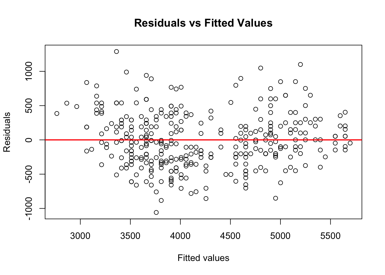

The following histogram of residuals suggests the residuals (and hence the error terms) are normally distributed

Show Code

lm_residuals <- simple_lm$residuals
h <- hist(lm_residuals,
          main = 'Distribution of Residuals',
          xlab = 'Residuals')
xfit <- seq(min(lm_residuals), max(lm_residuals), length = 40) 
yfit <- dnorm(xfit, mean = mean(lm_residuals), sd = sd(lm_residuals))
yfit <- yfit * diff(h$mids[1:2]) * length(lm_residuals) 
lines(xfit, yfit, col = "red", lwd = 2)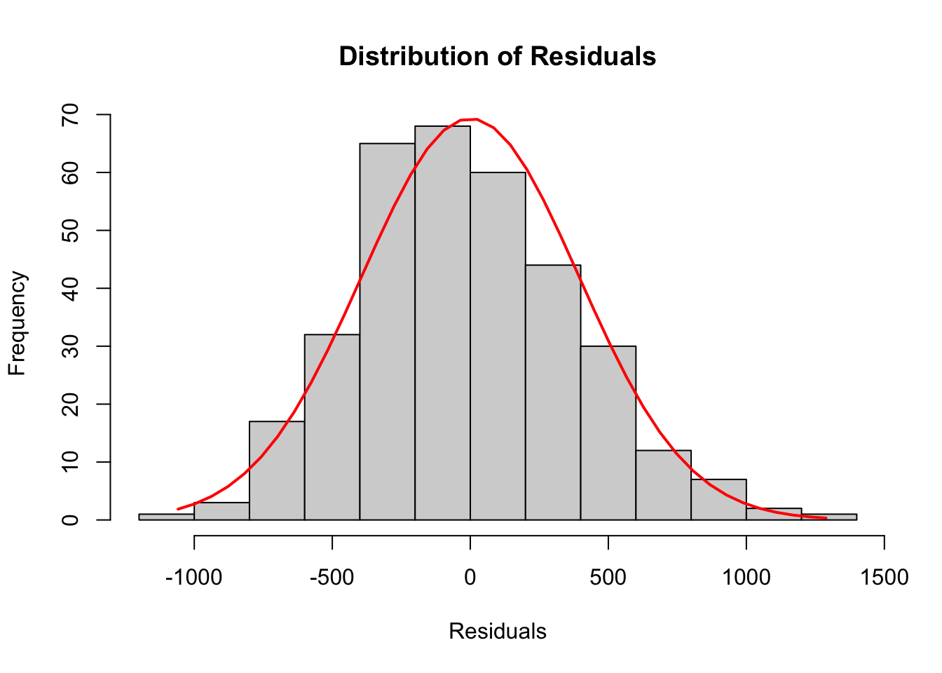

A more commonly used plot to test the normality of our residuals, is using a so-called Q-Q plot

qqnorm(simple_lm$residuals)
qqline(simple_lm$residuals)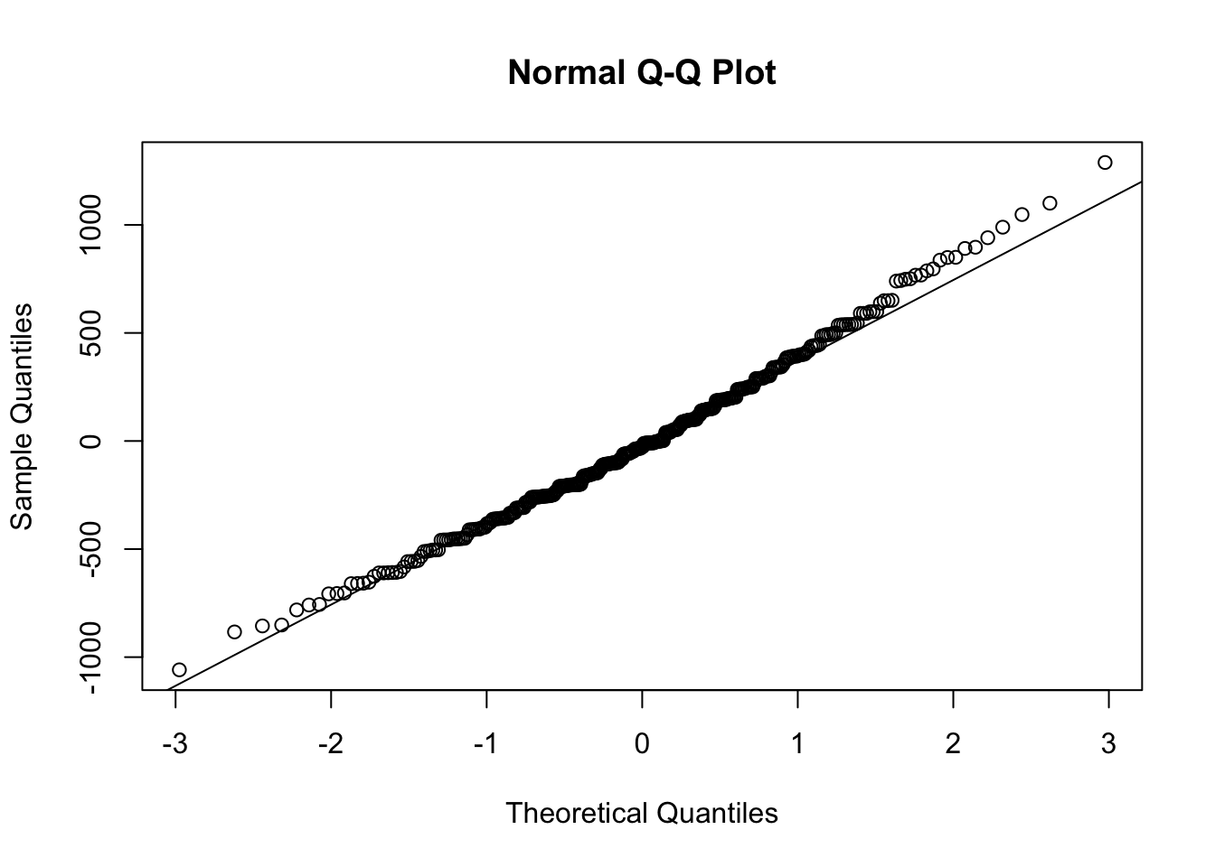 

To determine normality, if the residuals in the plot fall along the plotted line, then the data is normally distributed

Coefficients

Estimated regression beta coefficients \((\hat{\beta}_0, \hat{\beta}_1)\), alongside their standard errors, \(t\)-test, and \(p\)-values.

lm_summary$coefficients

                     Estimate Std. Error   t value      Pr(>|t|)
(Intercept)       -5780.83136 305.814504 -18.90306  5.587301e-55
flipper_length_mm    49.68557   1.518404  32.72223 4.370681e-107

From the output above:

• the model can be written as body_mass_g = -5780.831 + 49.686*flipper_length_mm

• the intercept \(\beta_0\) is -5780.831. It can be interpreted as the predicted body mass in grams for a flipper length of zero millimeters. In most scenarios the interpretation of the intercept coefficient will not make sense. For example, when the length of the flipper is zero millimeters we predict the weight of the penguin will be about -5780 grams

• the regression beta coefficient for the variable flipper_length_mm \(\beta_1\) is 49.686. That is, for each additional millimeter of the flipper we expect the penguin to gain 49.686 grams of body mass. For example, if the length of the flipper is 200 millimeters then we expect the penguin’s body mass to be about -5780.831 + 49.686 *200 = 4156.369 grams

Model Performance

Residual standard error (RSE), R-squared, Adjusted R-squared, and the F-statistic are metrics used to check our model performance. That is, how well does our model fit the data.

metrics <- c(lm_summary$sigma,lm_summary$r.squared,
             lm_summary$adj.r.squared,
             lm_summary$fstatistic['value'])

names(metrics) <- c('RSE','R_squared','Adj_R_squared','F_statistic')

metrics

          RSE     R_squared Adj_R_squared   F_statistic 
  394.2781775     0.7589925     0.7582837  1070.7445922 

Residual standard error

The average variation of the observations points around the fitted regression line. This is the standard deviation of residual errors The closer to this value is to zero the better.

R-squared/Adjusted R-squared

The proportion of information (i.e. variation) in the data that can be explained by the model. The adjusted R-squared adjusts for the degrees of freedom. The higher these values are the better.

In the simple linear regression setting R-squared is the square of the Pearson correlation coefficient

cor(flipper_length_mm,body_mass_g)^2

[1] 0.7589925

F-statistic

The F-statistic gives the overall significance of the model. It assess whether at least one predictor variable has a non-zero coefficient. The higher this value the better. However, this test only becomes more important when dealing with multiple predictors instead of a single predictor found in a simple linear regression.

Test of Significance for the Slope

The equation of the least squares regression line is given by \[ y = \beta_0 + \beta_1x \] where \(\beta_0\) and \(\beta_1\) minimize the sum of squared residuals

When the coefficients are estimated from data, we write the linear model as

\[ \hat{y} = \hat{\beta}_0 + \hat{\beta}_1x \]

Hence, a straightforward linear model encapsulates the linear correlation between two variables through two key summary statistics, namely \(\hat{\beta}_0\) and \(\hat{\beta}_1\). Specifically, \(\hat{\beta}_0\) serves as an estimate for the intercept, while \(\hat{\beta}_1\) provides an estimate for the slope of the linear model. The ‘hat’ symbols are employed when fitting the model to the data, often referred to as the “fitted model,” and \(\hat{y}\) represents the “fitted” or “predicted” values of the response variable

The primary objective in simple linear regression is often to understand the relationship between the independent variable and the dependent variable. The slope of the regression line represents the change in the dependent variable for a one-unit change in the independent variable. Therefore, testing the significance of the slope helps determine if there is a statistically significant linear relationship

\[ \begin{align*} H_0: \beta_1 = 0 \\ H_a: \beta_1 \neq 0 \end{align*} \]

Theory-based approach

A simple summary(lm()) call will perform a theory based approach for testing the statistical significance of the slope coefficient

simple_lm <- lm(body_mass_g ~ flipper_length_mm)

summary(simple_lm)

Call:
lm(formula = body_mass_g ~ flipper_length_mm)

Residuals:
     Min       1Q   Median       3Q      Max 
-1058.80  -259.27   -26.88   247.33  1288.69 

Coefficients:
                   Estimate Std. Error t value Pr(>|t|)    
(Intercept)       -5780.831    305.815  -18.90   <2e-16 ***
flipper_length_mm    49.686      1.518   32.72   <2e-16 ***
---
Signif. codes:  0 '***' 0.001 '**' 0.01 '*' 0.05 '.' 0.1 ' ' 1

Residual standard error: 394.3 on 340 degrees of freedom
Multiple R-squared:  0.759, Adjusted R-squared:  0.7583 
F-statistic:  1071 on 1 and 340 DF,  p-value: < 2.2e-16

Refer to SLR in R, for a more detailed explanation of the above output

Simulation-based approach

Below is a for loop that will simulate the null distribution for the slope of the regression line

iters <- 1000
slopes <- numeric(iters)
set.seed(123)

for (i in 1:iters){
flipperlength_shuffle_i <- sample(penguins_dat$flipper_length_mm)
    fit_i <- lm(body_mass_g ~ flipperlength_shuffle_i, data = penguins_dat)
    slopes[i] <- fit_i$coefficients[2]
}

Show Code

sampling_dist <- ggplot(data.frame(slopes),
                        aes(slopes))+
  geom_histogram(fill = 'steelblue',alpha = 0.3,
                 color = 'black',bins=30)+
  labs(title = 'Sampling distribution',
       subtitle = '',
       x = 'Slope Coefficients',y = '')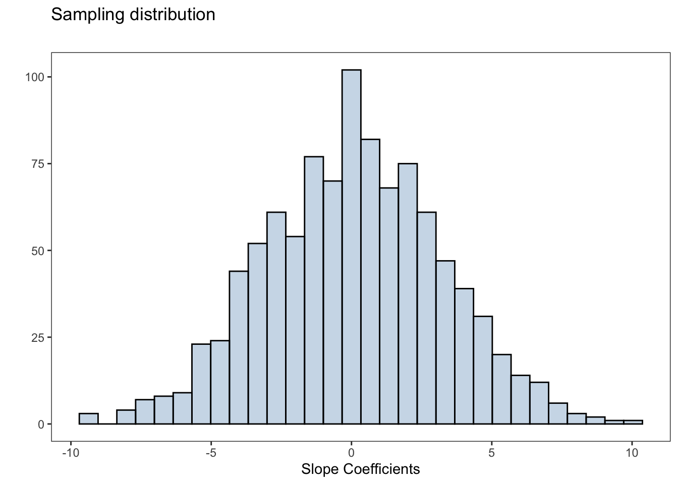

The \(p\)-value will be the proportion of times that the absolute value of the permuted statistics is greater than the absolute value of the observed statistic

obs_slope <- simple_lm$coefficients['flipper_length_mm']

mean(abs(slopes) >= abs(obs_slope))

[1] 0

The \(p\)-value is essentially zero, we have strong evidence to suggest the coefficient of the slope term is non-zero. That is, there is a statistically significant linear association between flipper length and the body mass of the penguins